nanoGPT-Models

Watching the nanoGPT series by Andrej Karpathy was really inspiring and the videos provided a really nice introduction to reproduce GPT-2 using the transformer architecture. In this post, I would like to document what I have learned from the Let’s build GPT: from scratch, in code, spelled out video.

The original transformer architecture was introduced in the Attention is all you need paper [1] as shown below.

Multi-Head Attention Mechanism

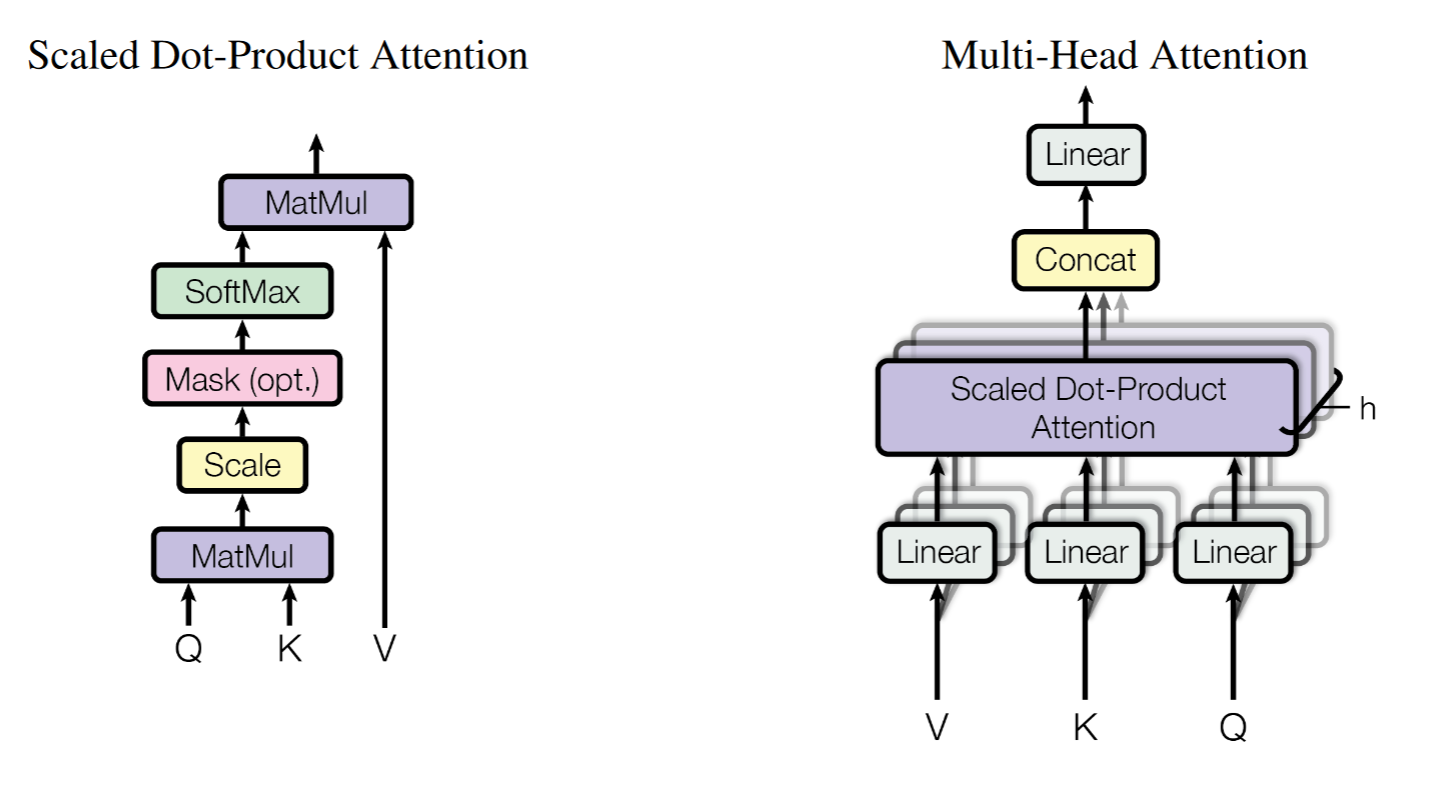
The self-attention mechanism from this paper was implemented as below from the nanoGPT repo:

class CausalSelfAttention(nn.Module):
    def __init__(self, config):
        super().__init__()
        assert config.n_embd % config.n_head == 0, "n_embd must be divisible by n_head!"
        # key, query, value projections for all heads, per batch
        self.c_attn = nn.Linear(config.n_embd, 3 * config.n_embd, bias=config.bias)
        # linear layer after concat all heads attention results
        self.c_proj = nn.Linear(config.n_embd, config.n_embd, bias=config.bias)
        
        self.n_embd = config.n_embd
        self.n_head = config.n_head
        # mask so that front token cannot query future tokens
        self.register_buffer("bias", torch.tril(torch.ones(config.block_size, config.block_size))
                                     .view(1, 1, config.block_size, config.block_size))

    def forward(self, x):
        B, T, C = x.shape # batch size, sequence length, embedding dimensionality (n_embd)

        q, k, v = self.c_attn(x).split(self.n_embd, dim=2)
        # Split to n_head for multiple heads, each head gets (T, hs) as input
        q = q.view(B, T, self.n_head, C // self.n_head).transpose(1, 2) # (B, nh, T, hs)
        k = k.view(B, T, self.n_head, C // self.n_head).transpose(1, 2) # (B, nh, T, hs)
        v = v.view(B, T, self.n_head, C // self.n_head).transpose(1, 2) # (B, nh, T, hs)

        att = (q @ k.transpose(-2, -1)) * (1.0 / math.sqrt(q.shape[-1])) # (B, nh, T, T)
        att = torch.masked_fill(att, self.bias[:,:,:T,:T] == 0, float('-inf'))
        att = F.softmax(att, dim=-1)
        y = att @ v # (B, nh, T, hs)
        y = y.transpose(1, 2).contiguous().view(B, T, C) # (B, T, C) rearrange number of heads together
        y = self.c_proj(y)
        return y

Takeaways

The dimensions

Here we have input to the multi-head attention (MHA) module as B x T x C, where B is the batch size, T is the sequence length, and C is the embedding size (same as d_model in the paper). For better efficiency, we put all W_Q, W_K and W_V together and matrix multiplication with our input and then split to get Q, K and V. Notice that we have broadcast mechanism comes to play for c_attn is broadcast to match the batch dimension.

We also have C = nh x hs where n_h is the number of heads and h_s is the head size. We must make sure embedding size is divisible by the number of heads. The transpose was used to make the scaled dot-product work so that each head will get the attention matrix of size T x T.

At the end of the foward function, after the matrix multiplication with V, the result was transposed and viewed to rearrange the layout to B x T x C again as the input for the next multi-head attention block.

Scaled dot-product

The $\sqrt{d_k}$ was used in scaled dot-product to add stability for the attention scores by preventing them become enormous. Condider the following property of variance: \[Var[aR]=a^2Var[R]\] If we have two vectors of unit Gaussian distribution $\mathcal{N}(0, 1)$, the variance of the dot product will be scaled up by the head size. Therefore, by dividing $\sqrt{d_k}$, we can make sure the variance of the dot product will be 1.

The mask

Inside self.register_buffer function we defined our mask to be a lower-triangular matrix, this is because in the decoder portion of the model, a front token should not be aware of or attend to the future tokens after it. For instance, the second token can see itself and the first token, but not the third token and afterwards. Therefore, for the second row of the attention matrix, we should set ‘-inf’ starting from the third element so that they will be equal to 0 when calculating the softmax.

self.register_buffer was used so that this mask is not considered as a model parameter which means torch will not keep calculating the gradient for it.

The linear layer

At the end of the multi-head self-attention block, we can find there is a linear layer after concatenating the results from all the heads. Here is my interpretation: before this linear layer, each token got a chance to know which token they are attended to but only given partial embedding. This linear layer gives the opportunity to communicate the information of the outputs from different heads with different embedding.

A complete MHA block

Below is the implementation for a comple MHA block:

class Layernorm(nn.Module):
    def __init__(self, ndim, bias):
        super().__init__()
        self.weight = nn.Parameter(torch.ones(ndim))
        self.bias = nn.Parameter(torch.zeros(ndim)) if bias else None

    def forward(self, x):
        return F.layer_norm(x, self.weight.shape, self.weight, self.bias, eps=1e-5)

class MLP(nn.Module):
    def __init__(self, config):
        super().__init__()
        self.n_embd = config.n_embd
        self.c_fc = nn.Linear(self.n_embd, 4 * self.n_embd)
        self.gelu = nn.GELU(approximate='tanh')
        self.c_proj = nn.Linear(4 * self.n_embd, self.n_embd)
    
    def forward(self, x):
        x = self.c_fc(x)
        x = self.gelu(x)
        x = self.c_proj(x)
        return x

class Block(nn.Module):
    def __init__(self, config):
        super().__init__()
        self.ln_1 = Layernorm(config.n_embd, config.bias)
        self.ln_2 = Layernorm(config.n_embd, config.bias)
        self.mlp = MLP(config)
        self.attn = CausalSelfAttention(config)
    
    def forward(self, x):
        # Use pre-norm here
        x = self.ln_1(x)
        x = x + self.attn(x)
        x = self.ln_2(x)
        x = x + self.mlp(x)
        return x

Layernorm

Layernorm is used instead of batchnorm due to the fact that T dimension can be different across the batch. For example, a long sentence versus a shor sentence. It is more meaningful to normalize across the embedding dimension for the case of language model. We have the so-called pre-norm fashion here which layernorm is applied before MHA, the original paper was applied after MHA.

Multi-layer perceptron

The MLP layer was used with GELU [2] activation function. GELU was used instead of ReLU [3] to reduce the “dead neuron” issue in the training phase. The MLP layer helps to add nonlinearity to the model.

Residual connection

The MHA blocks are stacked one by one and defined by N in the original paper. Therefore, the neuron network will get deeper with larger number of blocks. Residual connections [4] help to reduce the instability and diffcutiles when training very deep neuron networks.

Reference

[1] Vaswani, A., Shazeer, N., Parmar, N., Uszkoreit, J., Jones, L., Gomez, A. N., … & Polosukhin, I. (2017). Attention is all you need. Advances in neural information processing systems, 30.

[2] Hendrycks, D., & Gimpel, K. (2016). Gaussian error linear units (gelus). arXiv preprint arXiv:1606.08415.

[3] Vinod Nair and Geoffrey E. Hinton. 2010. Rectified linear units improve restricted boltzmann machines. In Proceedings of the 27th International Conference on International Conference on Machine Learning (ICML’10). Omnipress, Madison, WI, USA, 807–814.

[4] He, K., Zhang, X., Ren, S., & Sun, J. (2016). Deep residual learning for image recognition. In Proceedings of the IEEE conference on computer vision and pattern recognition (pp. 770-778).